
| 일 | 월 | 화 | 수 | 목 | 금 | 토 |
|---|---|---|---|---|---|---|
| 1 | 2 | 3 | 4 | 5 | ||
| 6 | 7 | 8 | 9 | 10 | 11 | 12 |
| 13 | 14 | 15 | 16 | 17 | 18 | 19 |
| 20 | 21 | 22 | 23 | 24 | 25 | 26 |
| 27 | 28 | 29 | 30 | 31 |
Tags
- 순환 신경망
- 풀링층
- 이미지 분류
- KONLPY
- 출력층
- 양방향 RNN
- 생성모델
- 코딩테스트
- 자연어 전처리
- 합성곱 신경망
- cnn
- 클러스터링
- COLAB
- 입력층
- 텍스트 마이닝
- RNN
- 과적합
- 임베딩
- 시계열 분석
- 원-핫 인코딩
- NLTK
- 프로그래머스
- 완전연결층
- 딥러닝
- 망각 게이트
- 전이학습
- 성능 최적화
- 합성곱층
- 코랩
- 카운트 벡터
Archives
- Today
- Total
Colab으로 하루에 하나씩 딥러닝
성능 최적화_2.드롭아웃을 통한 최적화 본문
728x90
드롭아웃(Dropout)
- 훈련할 때 일정 비율의 뉴런만 사용하고, 나머지 뉴런에 해당하는 가중치는 업데이트하지 않는 방법
- 노드를 임의로 끄면서 학습하는 방법으로, 은닉층에 배치된 노드 중 일부를 임의로 끄면서 학습
- 훈련 시간이 길어지는 단점이 있지만, 모델 성능을 향상하기 위해 자주 사용됨
드롭아웃 실습
### 라이브러리 호출

import tensorflow_datasets as tfds
import tensorflow as tf
### 데이터셋 내려받기
(train_data, test_data), info = tfds.load(
'imdb_reviews/subwords8k',
split=(tfds.Split.TRAIN, tfds.Split.TEST),
with_info=True, as_supervised=True) # 설명 1
padded_shapes=([None], ())
train_batches = train_data.shuffle(1000).padded_batch(10, padded_shapes=padded_shapes) # 설명 2
test_batches = test_data.shuffle(1000).padded_batch(10, padded_shapes=padded_shapes)
상세 설명
- 설명 1:
- tensorflow_datasets 라이브러리 중 load() 메서드 상세 내용
- 'imdb_reviews/subwords8k': 내려받을 데이터셋의 이름을 지정
- split: 내려받은 데이터셋을 훈련과 검증용으로 분리
- with_info=True: 전체 데이터에 대한 메타 정보도 함께 불러옴
- as_supervised=True: 데이터를 (input, label) 튜플 형태로 반환
- tensorflow_datasets 라이브러리 중 load() 메서드 상세 내용
- 설명 2:
- padded_batch() 메서드는 배치에서 가장 긴 문자열의 길이를 기준으로 시퀀스를 0으로 채움
### 데이터 배열로 변환

train_batch , train_labels = next(iter(train_batches))  # iter는 반복 가능한 객체에서 이터레이터를 반환하고, next는 이터레이터에서 값을 차례대로 꺼냄
train_batch.numpy() # 배열로 변환### 드롭아웃이 적용되지 않은 모델
encoder = info.features['text'].encoder
model = tf.keras.Sequential([
tf.keras.layers.Embedding(encoder.vocab_size, 64),
tf.keras.layers.LSTM(64),
tf.keras.layers.Dense(64, activation='relu'),
tf.keras.layers.Dense(1, activation='sigmoid')
]) # 설명 1상세 설명
- 설명 1:
- 임베딩층은 단어당 하나의 벡터를 저장
- 임베딩이 호출되면 단어 인덱스 시퀀스를 벡터 시퀀스로 변환
- 훈련 후 유사한 의미를 가진 단어는 종종 유사한 벡터를 가짐
### 모델 훈련

model.compile(loss='binary_crossentropy',
              optimizer=tf.keras.optimizers.Adam(1e-4), metrics=['accuracy'])
history = model.fit(train_batches, epochs=5, validation_data=test_batches, validation_steps=30)### 훈련 결과 시각화
import matplotlib.pyplot as plt
BUFFER_SIZE = 10000
BATCH_SIZE = 64
train_dataset = train_batches.shuffle(BUFFER_SIZE)
history_dict = history.history
acc = history_dict['accuracy']
val_acc = history_dict['val_accuracy']
loss = history_dict['loss']
val_loss = history_dict['val_loss']
epochs = range(1, len(acc)+1)
plt.figure(figsize=(4,3))
plt.plot(epochs, loss, 'bo', label='Training loss')
plt.plot(epochs, val_loss, 'b', label='Validation loss')
plt.title('Training and Validation loss')
plt.xlabel('Epochs')
plt.ylabel('Loss')
plt.legend()
plt.show()
plt.figure(figsize=(4,3))
plt.plot(epochs, acc, 'bo', label='Training acc')
plt.plot(epochs, val_acc, 'b', label='Validation acc')
plt.title('Training and Validation accuracy')
plt.xlabel('Epochs')
plt.ylabel('Accuracy')
plt.legend()
plt.ylim((0.5,1))
plt.show()
상세 설명
- 설명 1:
- 결과가 정상적이지 않음
- 테스트 데이터셋에 대한 손실/오차는 감소하는 추이를 보이지만 높음
- 테스트 데이터셋에 대한 정확도 0.6 보다 작아 매우 낮음
- 결과가 정상적이지 않음
### 드롭아웃이 적용된 모델

model = tf.keras.Sequential([
    tf.keras.layers.Embedding(encoder.vocab_size, 64),
    tf.keras.layers.Bidirectional(tf.keras.layers.LSTM(64, return_sequences=True)),
    tf.keras.layers.Bidirectional(tf.keras.layers.LSTM(32)),
    tf.keras.layers.Dense(64, activation='relu'),
    tf.keras.layers.Dropout(0.5),
    tf.keras.layers.Dense(1, activation='sigmoid')
])
model.summary()
### 모델 컴파일

model.compile(loss='binary_crossentropy',
              optimizer=tf.keras.optimizers.Adam(1e-4), metrics=['accuracy'])
history = model.fit(train_batches, epochs=5, validation_data=test_batches, validation_steps=30)
### 훈련에 대한 시각화

import matplotlib.pyplot as plt

BUFFER_SIZE = 10000
BATCH_SIZE = 64
train_dataset = train_batches.shuffle(BUFFER_SIZE)

history_dict = history.history
acc = history_dict['accuracy']
val_acc = history_dict['val_accuracy']
loss = history_dict['loss']
val_loss = history_dict['val_loss']
epochs = range(1, len(acc)+1)
plt.figure(figsize=(4,3))
plt.plot(epochs, loss, 'bo', label='Training loss')
plt.plot(epochs, val_loss, 'b', label='Validation loss')
plt.title('Training and Validation loss')
plt.xlabel('Epochs')
plt.ylabel('Loss')
plt.legend()
plt.show()

plt.figure(figsize=(4,3))
plt.plot(epochs, acc, 'bo', label='Training acc')
plt.plot(epochs, val_acc, 'b', label='Validation acc')
plt.title('Training and Validation accuracy')
plt.xlabel('Epochs')
plt.ylabel('Accuracy')
plt.legend(loc='lower right')
plt.ylim((0.5,1))
plt.show()
상세 설명
- 설명 1:
- 결과가 드롭아웃이 되기 전보다 향상됨
- 테스트 데이터셋에 대한 손실/오차는 감소하는 추이를 보이며 이전 결과보다 나음
- 테스트 데이터셋에 대한 정확도가 0.8 이상을 보이며 이전 결과보다 나음
- 결과가 드롭아웃이 되기 전보다 향상됨
드롭아웃을 제거하고 양방향 RNN만 적용했을 때, 성능 확인
### 양방향 RNN만 적용한 모델(드롭아웃과 성능 비교를 위해)

model = tf.keras.Sequential([
    tf.keras.layers.Embedding(encoder.vocab_size, 64),
    tf.keras.layers.Bidirectional(tf.keras.layers.LSTM(64)),
    tf.keras.layers.Dense(64, activation='relu'),
    tf.keras.layers.Dense(1, activation='sigmoid')
])
model.summary()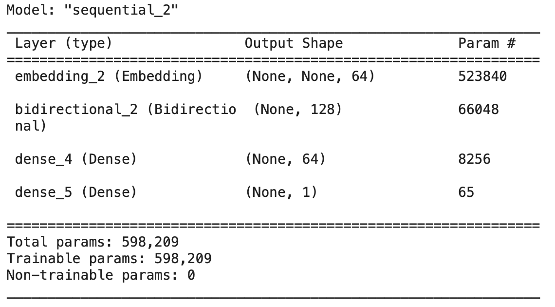
### 모델 훈련

model.compile(loss='binary_crossentropy',
              optimizer=tf.keras.optimizers.Adam(1e-4), metrics=['accuracy'])
history = model.fit(train_batches, epochs=5, validation_data=test_batches, validation_steps=30)
### 모델 훈련에 대한 시각화

import matplotlib.pyplot as plt

BUFFER_SIZE = 10000
BATCH_SIZE = 64
train_dataset = train_batches.shuffle(BUFFER_SIZE)

history_dict = history.history
acc = history_dict['accuracy']
val_acc = history_dict['val_accuracy']
loss = history_dict['loss']
val_loss = history_dict['val_loss']
epochs = range(1, len(acc)+1)
plt.figure(figsize=(4,3))
plt.plot(epochs, loss, 'bo', label='Training loss')
plt.plot(epochs, val_loss, 'b', label='Validation loss')
plt.title('Training and Validation loss')
plt.xlabel('Epochs')
plt.ylabel('Loss')
plt.legend()
plt.show()

plt.figure(figsize=(4,3))
plt.plot(epochs, acc, 'bo', label='Training acc')
plt.plot(epochs, val_acc, 'b', label='Validation acc')
plt.title('Training and Validation accuracy')
plt.xlabel('Epochs')
plt.ylabel('Accuracy')
plt.legend(loc='lower right')
plt.ylim((0.5,1))
plt.show()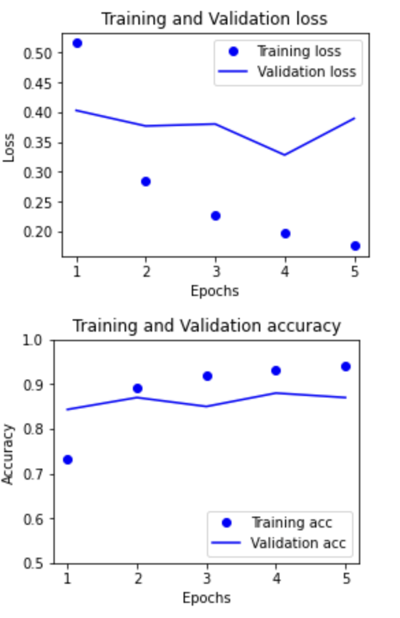
상세 설명
- 설명 1:
- 결과에 대한 리뷰
- 테스트 데이터셋에 대한 손실/오차가 높아지는 추이를 보임
- 테스트 데이터셋에 대한 정확도가 대략 0.9인 결과를 보임
- 결과에 대한 리뷰
참고: 서지영, 『딥러닝 텐서플로 교과서』, 길벗(2022)
'딥러닝_개념' 카테고리의 다른 글
| 클러스터링_1.K-평균 군집화 (0) | 2023.01.27 |
|---|---|
| 성능 최적화_3.조기 종료를 통한 최적화 (0) | 2023.01.26 |
| 성능 최적화_1.배치 정규화를 통한 최적화 (0) | 2023.01.21 |
| 시계열 분석_5.양방향 RNN (0) | 2023.01.19 |
| 시계열 분석_4.GRU (1) | 2023.01.18 |
'딥러닝_개념' Related Articles
more


