
| 일 | 월 | 화 | 수 | 목 | 금 | 토 |
|---|---|---|---|---|---|---|
| 1 | 2 | 3 | ||||
| 4 | 5 | 6 | 7 | 8 | 9 | 10 |
| 11 | 12 | 13 | 14 | 15 | 16 | 17 |
| 18 | 19 | 20 | 21 | 22 | 23 | 24 |
| 25 | 26 | 27 | 28 | 29 | 30 | 31 |
Tags
- 텍스트 마이닝
- 풀링층
- 성능 최적화
- 순환 신경망
- 생성모델
- 이미지 분류
- 양방향 RNN
- 완전연결층
- 합성곱 신경망
- cnn
- 카운트 벡터
- 과적합
- 클러스터링
- 원-핫 인코딩
- 딥러닝
- 코랩
- COLAB
- 시계열 분석
- 출력층
- 코딩테스트
- 망각 게이트
- 자연어 전처리
- 프로그래머스
- NLTK
- 임베딩
- 합성곱층
- RNN
- 입력층
- KONLPY
- 전이학습
Archives
- Today
- Total
Colab으로 하루에 하나씩 딥러닝
합성곱 신경망_3.전이학습_1) 특성 추출 기법 본문
728x90
전이학습 (Transfer learning)
- 아주 큰 데이터셋을 써서 훈련된 모델의 가중치를 가져와 해결하려는 과제에 맞게 보정
- 훈련을 시키기 위한 많은 양의 데이터, 돈과 시간을 절약함
- 전이학습 방법으로는 특성 추출과 미세 조정 기법이 있음
특성 추출 기법(Feature extractor)
- 학습할 때는 마지막 완전연결층 부분만 학습하고 나머지 계층들은 학습되지 않도록 함
- 이미지 분류를 위해 두 부분으로 나뉨
- 합성곱층: 합성곱층과 풀링층으로 구성
- 데이터 분류기(완전연결층): 추출된 특성을 입력받아 최종적으로 이미지에 대한 클래스를 분류하는 부분
- 사전 훈련된 네트워크의 합성곱층(가중치 고정)에 새로운 데이터를 통과시키고, 그 출력을 데이터 분류기에서 훈련시킴
특성 추출 기법 실습
### 라이브러리 호출

import numpy as np
import tensorflow as tf
import matplotlib.pyplot as plt
import matplotlib.image as mpimng

from tensorflow.keras import Model
from tensorflow.keras.models import Sequential
from tensorflow.keras.layers import Dense, GlobalMaxPool2D, GlobalAveragePooling2D
from tensorflow.keras.applications import ResNet50
from tensorflow.keras.preprocessing.image import ImageDataGenerator
### 사전 훈련된 모델 내려받기
model = ResNet50(include_top=True,
weights="imagenet",
input_tensor=None,
input_shape=None,
pooling=None,
classes=1000) # 설명 1상세 설명
- 설명 1:
- include_top: 네트워크 상단에 완전연결층을 포함하지 여부를 지정.(기본값은 True)
- weights: 가중치를 의미. 'None'(무작위 초기화) & 'imagenet'(ImageNet에서 사전 훈련된 값)
- input_tensor: 입력 데이터의 텐서
- input_shpae: 입력 이미지에 대한 텐서 크기
- pooling: 풀링에서 사용할 값 설정
- None: 마지막 합성곱층이 출력
- avg: 마지막 합성곱층에 글로벌 평균 풀링이 추가됨
- max: 마지막 합성곱층에 글로벌 최대 풀링이 추가됨
- classes: 'weights'로 'imagenet'을 사용하려면 classes값이 1000
### ResNet50 네트워크 구조 확인

model.summary()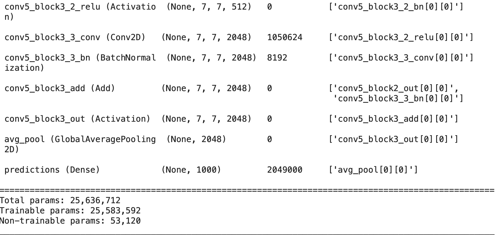
### ResNet50 네트워크에 밀집층 추가

model.trainable = False
model = Sequential([model,
                    Dense(2, activation='sigmoid')])  # 시그모이드 함수가 포함된 밀집층 추가
model.summary()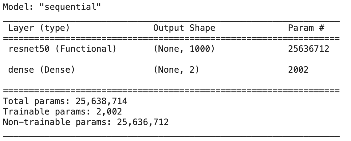
### 훈련에 사용될 환경 설정

model.compile(loss='binary_crossentropy',
              optimizer='adam',
              metrics=['accuracy'])
### git 클론을 통한 필요 데이터셋 로드
!git clone https://github.com/gilbutITbook/080263.git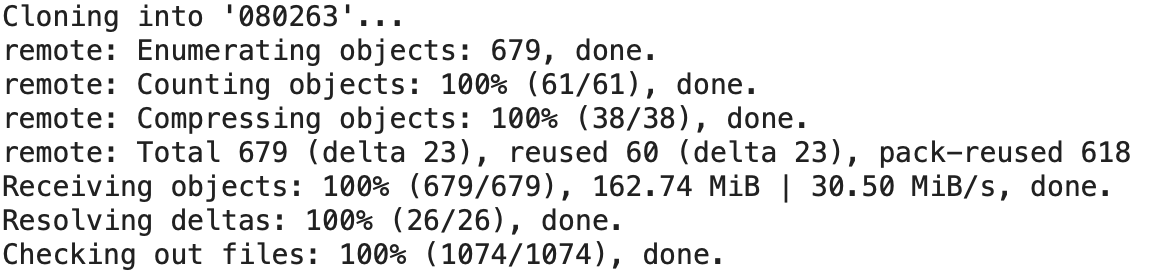
### 모델 훈련
BATCH_SIZE = 32
image_height = 224
image_width = 224
train_dir = "/content/080263/chap5/data/catanddog/train"
valid_dir = "/content/080263/chap5/data/catanddog/validation"
train = ImageDataGenerator(
rescale= 1./255,
rotation_range=10,
width_shift_range=0.1,
height_shift_range=0.1,
shear_range=0.1,
zoom_range=0.1) # 설명 1
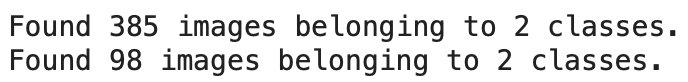
train_generator = train.flow_from_directory(train_dir,
target_size=(image_height, image_width),
color_mode="rgb",
batch_size=BATCH_SIZE,
seed=1,
shuffle=True,
class_mode="categorical") # 설명 2
valid = ImageDataGenerator(rescale=1.0/255.0)
valid_generator = valid.flow_from_directory(valid_dir,
target_size=(image_height, image_width),
color_mode="rgb",
batch_size=BATCH_SIZE,
seed=7,
shuffle=True,
class_mode="categorical")
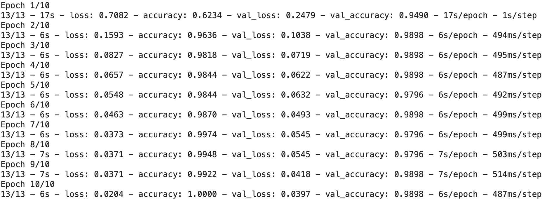
history = model.fit(train_generator,
epochs=10,
validation_data=valid_generator,
verbose=2) # 설명 3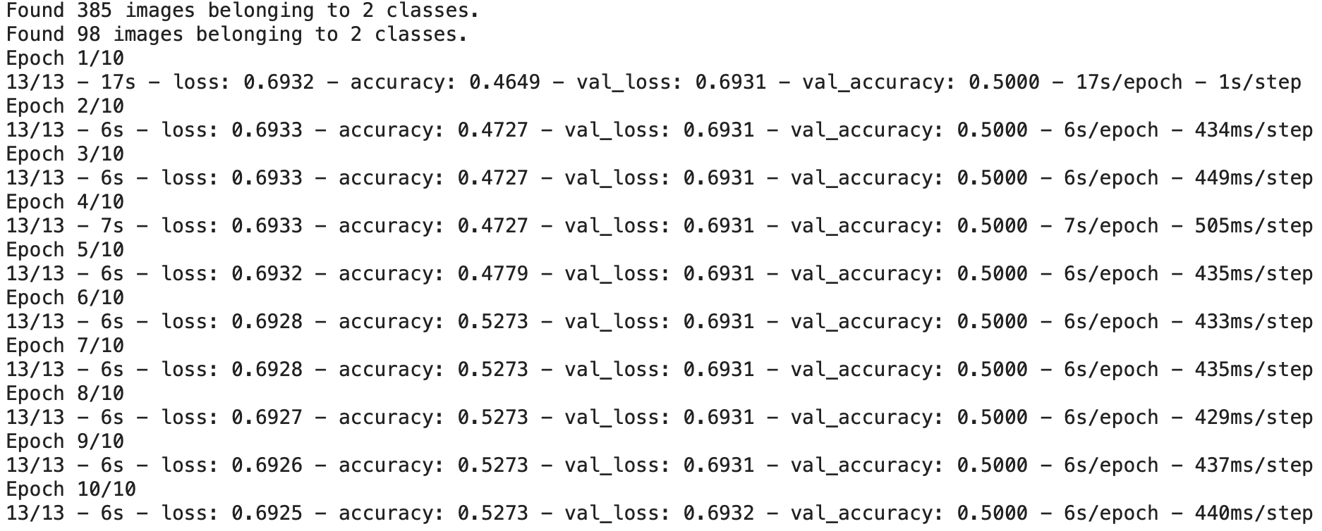
상세 설명
- 설명 1:
- rescale: 원본 이미지는 0~255의 RGB 계수로 구성됨. 1/255로 스케일링하여 0~1 범위로 변환
- rotation_range: 이미지 회전 범위
- rotation_range=10 이면, 0~10도 범위 내에서 임의로 원본 이미지를 회전
- width_shift_range: 그림을 수평으로 랜덤 하게 평행 이동시키는 범위
- width_shift_range=0.1이면, 전체 넓이가 10일 경우 1픽셀 내외로 이미지를 좌우로 이동
- height_shift_range: 그림을 수직으로 랜덤하게 평행 이동시키는 범위
- height_shift_range=0.1이면, 전체 높이가 10일 경우 1픽셀 내외로 이미지를 상하로 이동
- shear_range: 원본 이미지를 임의로 변환 시키는 범위
- shear_range=0.1이면, 0.1 라디안 내외로 시계 반대 방향으로 이미지를 변환
- zoom_range: 임의 확대/축소 범위
- zoom_range=0.1이면, 0.9에서 1.1배의 크기로 이미지 변환
- 설명 2:
- train_dir: 훈련 이미지 경로
- target_size: 이미지 크기, 모든 이미지는 이 크기로 자동 조정됨
- color_mode: 이미지가 흑백이면 'grayscale', 색상이 있으면 'rgb'
- batch_size: 배치당 generator에서 생성할 이미지 개수
- seed: 이미지를 임의로 섞기 위한 랜덤한 숫자
- shuffle: 이미지를 섞어서 사용하면 'True', 섞지 않는다면 'False'
- class_mode: 예측할 클래스가 두개면 'binary', 세 개 이상이면 'categorical'
- 설명 3:
- train_dir: 학습에 사용되는 데이터셋
- epochs: 학습에 대한 반복 횟수
- validation_data: 테스트 데이터셋 설정
- verbose: 훈련의 진행 과정을 보여줌
- 0: 아무것도 출력하지 않음
- 1: 훈련의 진행도를 표시하는 진행 막대를 보여줌
- 2: 미니 배치마다 훈련 정보를 출력
### 모델의 정확도 시각화

import matplotlib as mpl
import matplotlib.pylab as plt
from matplotlib import font_manager

accuracy = history.history['accuracy']	# 설명 1
val_accuracy = history.history['val_accuracy']

loss = history.history['loss']
val_loss = history.history['val_loss']

epochs = range(len(accuracy))

plt.plot(epochs, accuracy, label="훈련 데이터셋")
plt.plot(epochs, val_accuracy, label="검증 데이터셋")
plt.legend()
plt.title('정확도')
plt.figure()

plt.plot(epochs, loss, label="훈련 데이터셋")
plt.plot(epochs, val_loss, label="검증 데이터셋")
plt.legend()
plt.title("오차")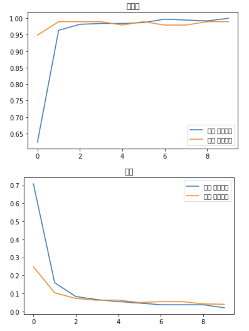
상세 설명
- 설명 1:
- accuracy: 매 에포크에 대한 훈련의 정확도를 나타냄
- loss: 매 에포크에 대한 훈련의 손실 값을 나타냄
- val_accuracy: 매 에포크에 대한 검증의 정확도를 나타냄
- val_loss: 매 에포크에 대한 검증의 손실 값을 나타냄
### 훈련된 모델의 예측

class_names = ["cat", "dog"]	# 개와 고양이에 대한 클래스 두개
validation, label_batch = next(iter(valid_generator))	# 설명 1
prediction_values = model.predict(validation)
prediction_values = np.argmax(prediction_values, axis=1)

fig = plt.figure(figsize=(12,8))
fig.subplots_adjust(left=0, right=1, bottom=0, top=1, hspace=0.05, wspace=0.05)

for i in range(8):	# 이미지 여덟 개에 대한 출력
  ax = fig.add_subplot(2, 4, i+1, xticks=[], yticks=[])
  ax.imshow(validation[i,:], cmap=plt.cm.gray_r, interpolation='nearest')
  if prediction_values[i] == np.argmax(label_batch[i]):
    ax.text(3, 17, class_names[prediction_values[i]], color='yellow', fontsize=14)
  else:
    ax.text(3, 17, class_names[prediction_values[i]], color='red', fontsize=14)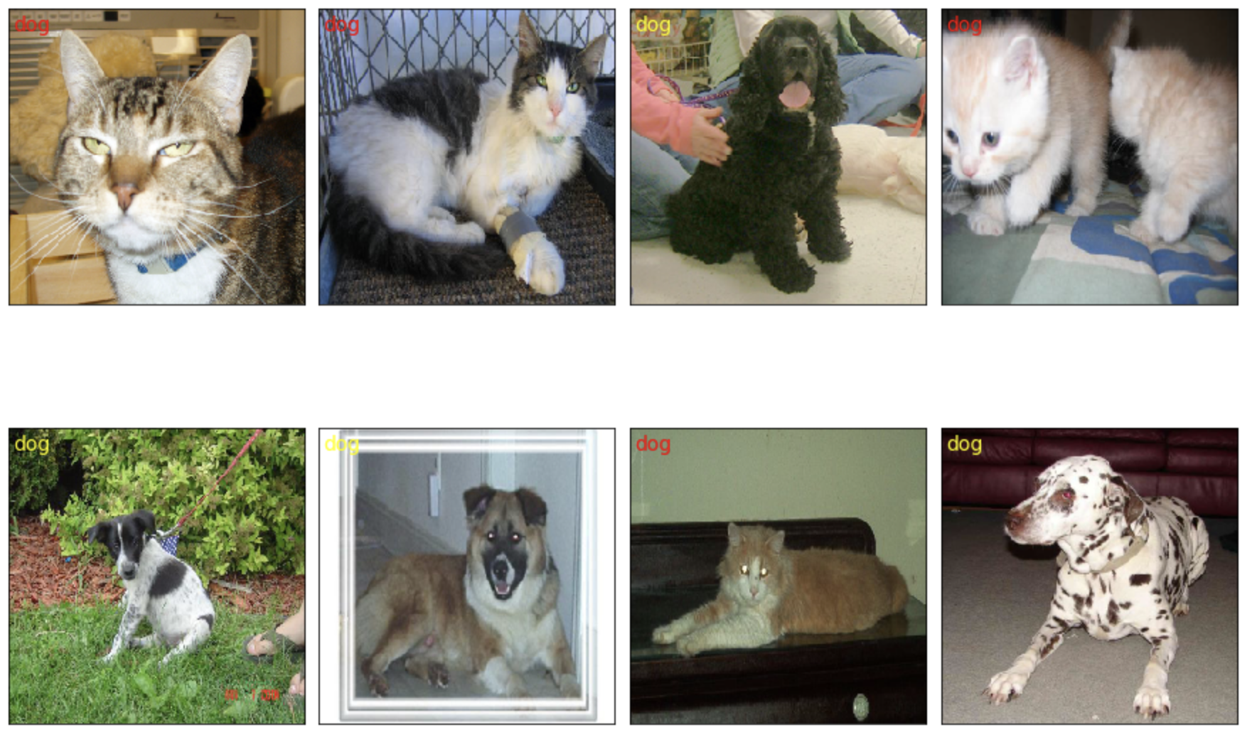
상세 설명
- 설명 1:
- iter() 메서드와 next() 메서드가 있어야 반복자(iterator)를 사용할 수 있음
- iter(): 전달된 데이터의 반복자를 꺼내 반환
- next(): 반복자를 입력으로 받아 그 반복자가 다음에 출력해야할 요소를 반환
- iter() 메서드와 next() 메서드가 있어야 반복자(iterator)를 사용할 수 있음
### 텐서플로 허브에서 라이브러리 호출 및 ResNet50 내려받기

import tensorflow_hub as hub
model = tf.keras.Sequential([
    hub.KerasLayer("https://tfhub.dev/google/imagenet/resnet_v2_152/feature_vector/4",
                   input_shape=(224,224,3),
                   trainable=False),
                   tf.keras.layers.Dense(2, activation='softmax')
])
### 데이터 확장
train = ImageDataGenerator(
rescale=1./255,
rotation_range=10,
width_shift_range=0.1,
height_shift_range=0.1,
shear_range=0.1,
zoom_range=0.1)
train_generator = train.flow_from_directory(train_dir,
target_size=(image_height, image_width),
color_mode="rgb",
batch_size=BATCH_SIZE,
seed=1,
shuffle=True,
class_mode="categorical")
valid = ImageDataGenerator(rescale=1.0/255.0)
valid_generator = valid.flow_from_directory(valid_dir,
target_size=(image_height, image_width),
color_mode="rgb",
batch_size=BATCH_SIZE,
seed=7,
shuffle=True,
class_mode="categorical")
model.compile(loss='binary_crossentropy',
optimizer='adam',
metrics=['accuracy'])
### 모델 훈련

history = model.fit(train_generator,
                    epochs=10,
                    validation_data=valid_generator,
                    verbose=2)
### 모델의 정확도를 시각적으로 표현

accuracy = history.history['accuracy']
val_accuracy = history.history['val_accuracy']

loss = history.history['loss']
val_loss = history.history['val_loss']

epochs = range(len(accuracy))

plt.plot(epochs, accuracy, label="훈련 데이터셋")
plt.plot(epochs, val_accuracy, label="검증 데이터셋")
plt.legend()
plt.title('정확도')
plt.figure()

plt.plot(epochs, loss, label="훈련 데이터셋")
plt.plot(epochs, val_loss, label="검증 데이터셋")
plt.legend()
plt.title('오차')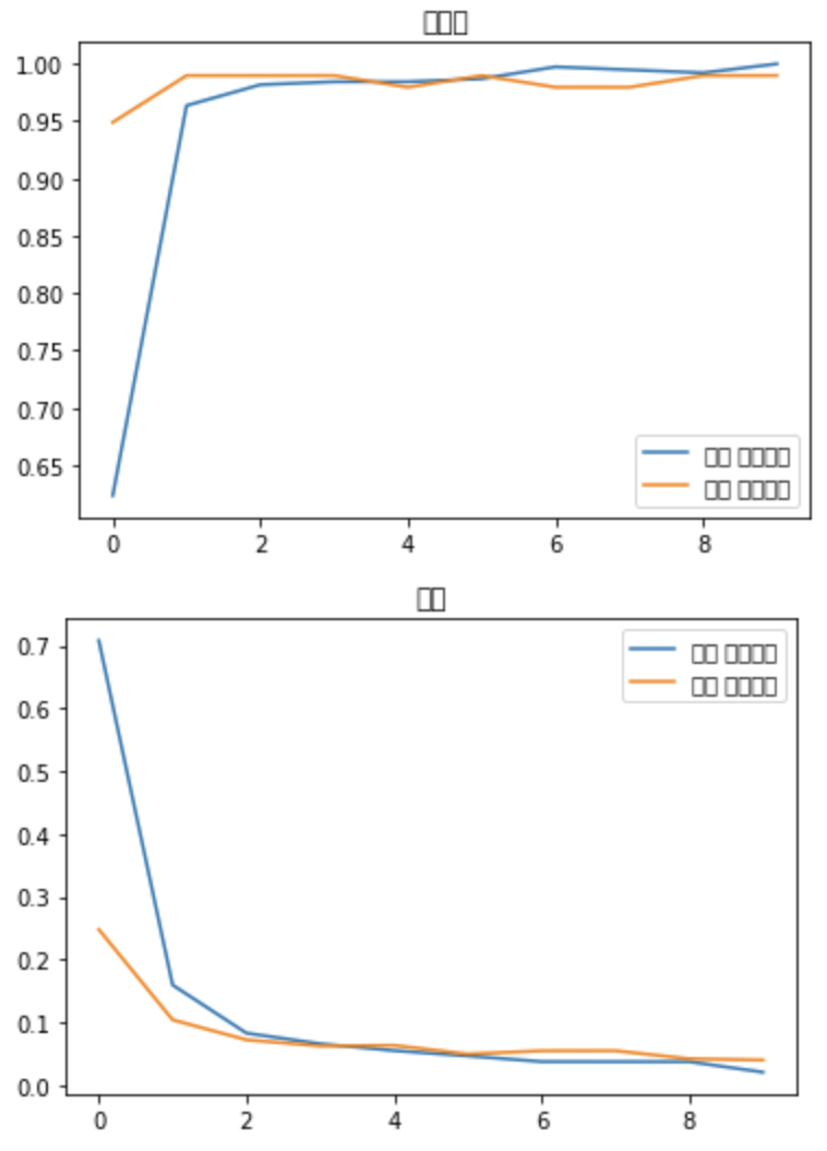
### 이미지에 대한 예측 확인

class_names=['cat', 'dog']
validation, label_batch = next(iter(valid_generator))
prediction_values = model.predict(validation)
prediction_values = np.argmax(prediction_values, axis=1)

fig = plt.figure(figsize=(12,8))
fig.subplots_adjust(left=0, right=1, bottom=0, top=1, hspace=0.05, wspace=0.05)

for i in range(8):
  ax = fig.add_subplot(2,4, i+1, xticks=[], yticks=[])
  ax.imshow(validation[i,:], cmap=plt.cm.gray_r, interpolation='nearest')
  if prediction_values[i] == np.argmax(label_batch[i]):
    ax.text(3,17, class_names[prediction_values[i]], color='yellow', fontsize=14)
  else:
    ax.text(3,17,class_names[prediction_values[i]], color='red', fontsize=14)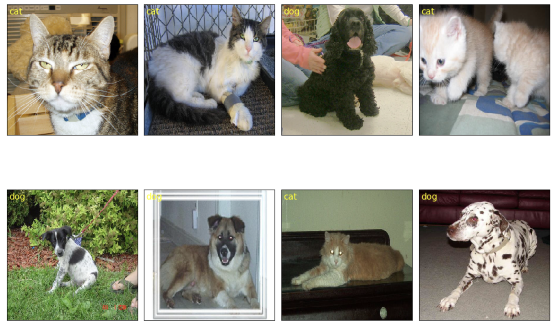
참고: 서지영, 『딥러닝 텐서플로 교과서』, 길벗(2022)
'딥러닝_개념' 카테고리의 다른 글
| 합성곱 신경망_4.CNN 시각화 (0) | 2023.01.05 |
|---|---|
| 합성곱 신경망_3.전이학습_2) 미세 조정 기법 (0) | 2023.01.04 |
| 합성곱 신경망_2.fashion_mnist 실습 (0) | 2022.12.28 |
| 합성곱 신경망_1.CNN이란? (1) | 2022.12.27 |
| 텍스트 마이닝_ 1. BOW 기반의 텍스트 마이닝_4)로지스틱 회귀분석 (1) | 2022.12.26 |
'딥러닝_개념' Related Articles
more

